SVD를 활용한 이미지 압축: 특이값 분해

SVD: Singular Vector Decomposition에 대해 다룬다. 각 수식이 어떤 의미를 가지고, 이미지 압축에 어떻게 사용되는지 설명한다. 본 글을 이해하기 위해 아래 개념을 이해하고 있어야 한다.

Vector: 크기와 방향을 가지는 양으로, 2차원 공간의 벡터는 $\overrightarrow{v}=\left[\begin{array}{cc}{u}_1& u_2\end{array}\right]$와 같이 표현한다. 본문에서는 $v$ 형태로 표기한다.

Inversed matrix: $A$에 대한 역행렬로 $A^{-1}$로 표기하며, $A^{-1}A=I$라는 특징을 가진다.

Orthogonal matrix: 모든 column 벡터가 직교하는 행렬로, $A{A}^T=A^{T}A=I$라는 특징을 가진다. 동시에 $A^T=A^{-1}$이다.

Diagonal matrix: 주대각 성분을 제외한 모든 값이 0으로 $diag(u_1,u_2)=\left[\begin{array}{cc}{u}_1& 0\\ 0& u_2\end{array}\right]$와 같은 형태를 가진다.

선형 변환: $s\cdot \overrightarrow{v}$를 통해 벡터의 크기를 왜곡할 수 있다. 이미지 변환 중 "크기 변환" 참고.

---

Eigenvector의 특징

eigenvector는 고윳값으로 불리며, 선형 변환이 발생해도 방향을 유지하는 벡터를 말한다. eigenvector를 검색하면 다음과 같은 식이 나온다.

$$Av=\lambda v$$

식만 봐서는 모르겠으니, 한 단계씩 해석해 보자. $Av$는 벡터 $v$에 행렬 $A$를 곱해 선형 변환을 했다. 이 과정에서 대부분의 벡터는 왜곡된다.

$$Av=\left[\begin{array}{cc}2& 1\\ 1& 3\end{array}\right]v$$

하지만 같은 방향을 유지하는 벡터도 존재한다. 이 벡터를 eigenvector라고 부른다. 방향은 유지하고 있지만 크기는 바뀌었다. 따라서, 변형된 벡터를 $\lambda v$로 표현할 수 있다. $\lambda$는 크기를 조절하는 scaling factor 역할을 한다. eigenvector의 크기를 결정하는 $\lambda$를 eigenvalue라고 한다.

>>> eigenvalues, eigenvectors = np.linalg.eig(transformation_matrix)
>>> eigenvectors
[[-0.85065081 -0.52573111]
 [ 0.52573111 -0.85065081]] 
>>> eigenvalues
[1.38196601 3.61803399]

다시 처음으로 돌아와 $Av=\lambda v$는 벡터 $v$에 $A$를 통해 선형 변환을 해도 여전히 $v$인 0이 아닌 벡터를 eigenvector라고 한다. 이때 eigenvector에 곱해진 scaling factor를 eigenvalue라고 한다.

행렬 재구성

eigenvector와 eigenvalue를 알면, 변환 행렬 $A$를 찾을 수 있다.

$$A=V\mathrm{\Sigma }{V}^{-1}$$

$V$는 각 열이 eigenvector인 행렬이다. $\mathrm{\Sigma }=diag(...eigenvalue)$로 eigenvalue를 담고 있는 diagonal matrix이다.

다시 말해, 행렬 A는 eigenvector와 eigenvalue로 분해할 수 있고, 이 값들을 통해 재구성할 수 있다. 이 개념이 이미지를 압축하고 재구성하는 과정에도 적용된다. 하지만 eigenvector는 n x n의 square matrix에만 적용 가능하다. 따라서 eigenvector 대신 singular vector가 등장한다.

---

SVD

orthogonal matrix $U$와 $V$에 대해 아래 식이 성립한다.

$$A=U\mathrm{\Sigma }{V}^T$$

$A$는 m x n 크기의 행렬이며, $\mathrm{\Sigma }$는 diagonal matrix이다. 식을 정리해 보면 다음과 같다.

$$AV=U\mathrm{\Sigma }$$

이번에는 orthogonal matrix $V$와 선형 변환해도 여전히 orthogonal 한 $U$를 찾는 문제다.

식을 조금 더 정리해보면,

$$A{A}^T=U\mathrm{\Sigma }{V}^T(V{\mathrm{\Sigma }}^T{U}^T)$$

$$A{A}^T=U({\mathrm{\Sigma }}^T\mathrm{\Sigma })U^T$$

글 초반에 소개했던 행렬의 특성을 이용해 정리한 식이다. 위 식을 행렬로 시각화하면 다음과 같다.

눈치챘다시피 $U$는 eigenvector와 동일하다. ${\mathrm{\Sigma }}^T\mathrm{\Sigma }$는 diagonal matrix로 eigenvalue와 동일하다.

식을 $V$에 대해 정리하면,

$$A^{T}A=V({\mathrm{\Sigma }}^T\mathrm{\Sigma })V^T$$

따라서 $V$도 eigenvector와 같은 성질을 가진다.

용어 정리

$U$와 $V$는 singular vector로 eigenvector와 같은 의미를 가진다. $\mathrm{\Sigma }$는 singular value로 eigenvalue와 동일하다.

$$A=U\mathrm{\Sigma }{V}^T$$

• $U$: Left Singular Vector
• $V$: Right Singular Vector
• $\mathrm{\Sigma }$: Singular Value

정리하면, $A$는 singular vector $U$와 $V$로 분해되며, $\mathrm{\Sigma }$는 scaling 정도를 나타내는 singular value이다.

A = np.array([[1, 2], [3, 4], [5, 6]])

# Perform SVD (A = U * Σ * V^T)
U, sigma, Vt = np.linalg.svd(A)

---

이미지 분해

이미지 가로 길이가 $w$, 세로 길이가 $h$일 때, 2차원 이미지는 $h\times w$ 행렬로 표현할 수 있다. 이미지 행렬을 $M$라고 할 때, 이미지는 다음과 같이 분해할 수 있다.

$$M=U\mathrm{\Sigma }{V}^T$$

$$U=[u_1,u_2...u_h]$$

$$V=[v_1,v_2...v_w]$$

$$\mathrm{\Sigma }=diag({\sigma }_1,{\sigma }_2,...{\sigma }_n)$$

SVD에 재밌는 특징이 있는데 singular value가 큰 값부터 내림차순으로 나열되어 있다는 점이다.

$\sigma$ 중 ${\sigma }_1$이 가장 큰 값을 갖는다. 즉, 첫 번째 값부터 순서대로 중요한 정보를 담고 있다.

이미지 행렬 $M$은 $\sum _{n=1}{\sigma }_n{u}_n{v}_n^T$으로 표현할 수 있다. 그런데 만약 정보를 전부 사용하지 않고, 중요한 정보 몇 가지만 사용하면 어떨까?

가로 500, 세로 600의 600 x 500 행렬에 대해 실험을 해보았다.

당연히 벡터를 많이 사용할수록 이미지가 선명해진다.

singular value를 시각화해보면 n = 184에서 이미 singular value 총합의 80%를 넘어간다. 184개의 singular vector만으로도 이미지의 80%를 복원할 수 있다.

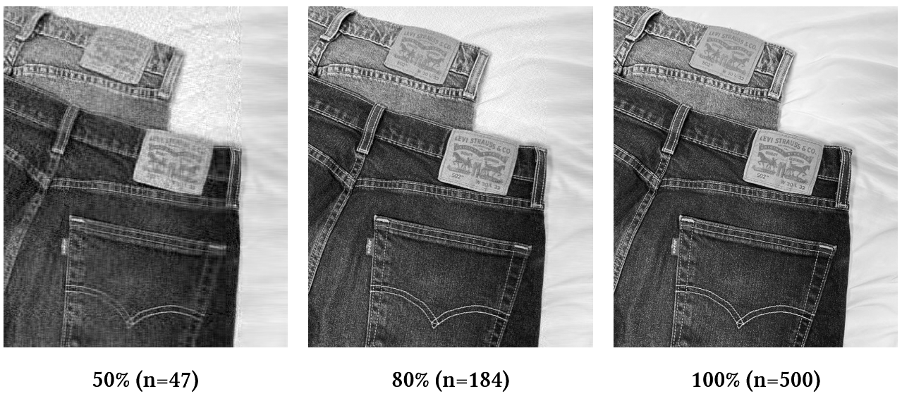
만약 600 x 500 행렬을 모두 사용하면 총 300,000개의 정보가 필요하다. 하지만, n = 200이라면 600 * n + n + n * 500으로 총 220,200개의 정보만 있으면 된다. 

따라서, SVD를 이용해 정보를 압축할 수 있다.

SVD 관련 코드

SVD는 np.linalg.svd를 통해 계산한다. full_matrices 옵션은 불필요한 벡터를 저장할지 결정한다.

"""이미지 분해 및 재구성"""

import numpy as np
from PIL import Image
import os

image_path = "object4.jpg"
output_dir = "svd_images"

image = Image.open(image_path).convert("L")
image = np.array(image, dtype=np.float64)

# Singular Vector Decomposition (SVD)
# Image: (600, 500), S: (500,), Vt: (500, 500)
# U: (600, 500) when full_matrices=False
# U: (600, 600) when full_matrices=True
U, S, Vt = np.linalg.svd(image, full_matrices=False)

# 이미지 재구성
for n in range(1, len(S) + 1):
    singular_values = np.zeros((U.shape[1], Vt.shape[0]))
    np.fill_diagonal(singular_values, S[:n])
    reconstructed = np.dot(
        U[:, :n],
        np.dot(singular_values[:n, :n], Vt[:n, :]),
    )
    output_image = np.clip(reconstructed, 0, 255).astype(np.uint8)

    # 단계별 이미지 저장
    if n % 10 == 0:
        output_path = os.path.join(output_dir, f"{n}.png")
        Image.fromarray(output_image).save(output_path)

"""Singular value 시각화"""

from PIL import Image
import numpy as np
import matplotlib.pyplot as plt

image = Image.open("object4.jpg").convert("L")
image = np.array(image, dtype=np.float64)

U, S, Vt = np.linalg.svd(image, full_matrices=False)

cumulative_sum = np.cumsum(S)
total_sum = np.sum(S)
threshold_percentage_1 = 0.5
threshold_percentage_2 = 0.8
threshold_1 = total_sum * threshold_percentage_1
threshold_2 = total_sum * threshold_percentage_2

threshold_index_1 = np.argmax(cumulative_sum >= threshold_1)
threshold_index_2 = np.argmax(cumulative_sum >= threshold_2)

plt.figure(figsize=(14, 6))
plt.plot(range(len(S)), S, label="Values")
plt.axvline(
    x=threshold_index_1,
    color="lightcoral",
    linestyle="--",
    label=f"{threshold_percentage_1 * 100}% Threshold (Index: {threshold_index_1})",
)
plt.axvline(
    x=threshold_index_2,
    color="red",
    linestyle="--",
    label=f"{threshold_percentage_2 * 100}% Threshold (Index: {threshold_index_2})",
)

plt.xlabel("Index")
plt.ylabel("Singular value")
plt.ylim(0, S[0] + 1)
plt.legend()
plt.grid(True)
plt.show()

---

참고자료

• 3Blue1Brown: 고유벡터와 고유값
• MIT OpenCourseWare: SVD